Neural Style Transfer in a Nutshell

Learn what makes this fascinating technology work.
Introduction
Neural Style Transfer (NST) is a technique where the style of one image is applied to another one while the content of the original image is kept. The result is a combined image of the content from the content image painted or drawn in the style of the style image. Probably the most famous example used to demonstrate style transfer is van Gogh’s Starry Night. Look at the pictures below and see how the style of Starry Night has been applied to the content image:
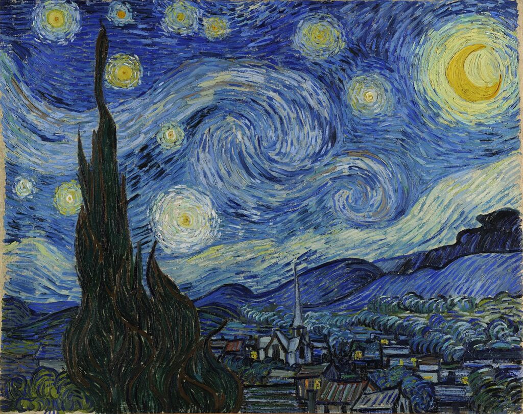
Style Image 
Content Image 
Stylized Image
Enthusiasts around the world have applied the style of van Gogh’s masterpiece to many of their own pictures. Let’s face it, not everyone is a born artist, and getting some help from the old masters is much appreciated. The resulting images can be used for decorations, as a profile picture, or in marketing and advertisement. It is even possible to paint a whole movie in a certain style by stylizing it frame by frame.
Neural style transfer (NST)
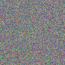
The technique of neural style transfer was first published in Leon A. Gatys’ paper, A Neural Algorithm of Artistic Style in 2015. His version of neural style transfer uses a feature extraction network and 3 images, a content image, a style image, and an input image. Think of the input image as a blank canvas that will become the stylized image during the process. At the very beginning, the input image is initialized with white noise. That is, every pixel in the image has a random color. The feature extraction network is a pre-trained image classification network that contains several convolutional layers.
How Neural Style Transfer Works
- At first the
style imageruns through thefeature extraction networkand the style values are measured and saved. - Then, the
content imageruns through thefeature extraction networkand the content values are measured and saved. - Now an iterative process starts:
- The input image runs through the
feature extraction network. - The content and style values are measured and compared to the saved content and style values from before.
- From the measured values and the saved values the
content lossandstyle lossare being calculated. - The
content lossandstyle lossare being combined into atotal loss. - An optimizing algorithm such as
stochastic gradient descent(SGD) is used to optimize the input image pixel by pixel. - The iterative process continues until the
total lossvalue saturates.
- The input image runs through the
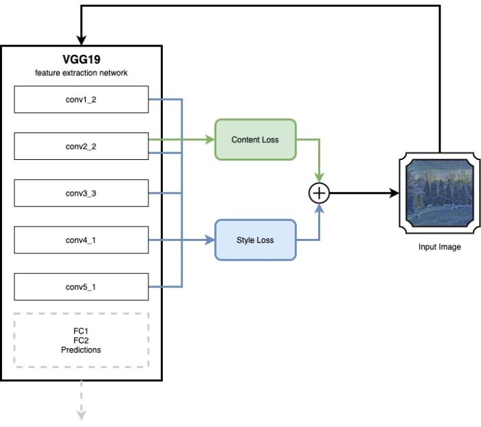
The result is a single stylized image. The diagram below shows the stylizing process of an image after the content and style baselines have been determined:
Feature Extraction Network
What makes style transfer so interesting (besides the awesome pictures it can create) is how it demonstrates the capabilities and internal representations of neural networks. As we have seen in the example above, the feature extraction network plays an important role to determine the content and style values for an image. The feature extraction network is a pre-trained image classifier. The classifier’s weights are frozen during the styling process. That means, there is no training of the network at all. A classifier that is often used in style transfer is the VGG19 that is trained on ImageNet with 1000 classes. The straight forward architecture of the VGG networks makes them a good candidate for style transfer applications. The VGG networks have several CNN layers on top of each other with no shortcuts in between them.
The image classifier contains many convolutional layers that are great for detecting patterns and objects in images. While the first layers tend to learn low-level features such as edges or corners, the deeper layers learn more and more complex structures. The last few layers in VGG19 (FC1, FC2 and softmax) are needed for classification and don’t have a use in style transfer. It is save to leave them out.
When an image runs through the network, the activation in the convolutional layers can be used to measure content and style of an image. The content and style loss is then calculated in comparison with the content and style values determined for the content and style image.
Content Loss
When an image runs through the network, it will activate filters in the convolutional layers. The content values are then measured as the activations of each filter in a convolutional layer. The content loss is calculated by the Euclidean Distance between the input image’s measured content values, and the content image’s saved values. If two images activate the same features in the network, their content must be similar.
The content loss can be calculated as follows:
L_{content} = \sum_{l}\sum_{i,j}(\alpha C_{i,j}^{s, l} - \alpha C_{i,j}^{c, l})^2
But what values are actually used in this equation, where do they come from? The alpha is just a hyper parameter to control how much weight the content loss shall have in the total loss. The l is the CNN layer in the VGG network. The i is the feature map channel, that is each feature map in a CNN layer creates a channel. The j is the position in the channel.
Experiments have shown that taking the activations from block2, layer2 (or conv2_2 for short) generate good results.
Style Loss
To derive the style loss things get a bit more complex but the principle is actually the same. A style value is derived from feature activations in multiple convolutional layers. The style loss then is calculated from this value and the saved values of the style image using a Gram matrix.
The Gram Matrix is defined as follow:
G_{i,k}^l = \sum_{k} F_{i,k}^l F_{j,k}^l
Below is an example how the Gram matrix is derived for layer 2. The same is done for a few more layers in the VGG network to calculate the total style loss.
Once the Gram matrix is calculated the style loss can be computed from the Gram matrix of the current image and the Gram matrix that has been determined from the style image at the beginning:
L_{style} = \sum_{l}\sum_{i,j}(\beta G_{i,j}^{stylized,l} - \beta G_{i,j}^{style,l})^2
Experiments have shown that taking the activations from conv1_2, conv2_2, conv3_3, conv4_1 and conv5_1 generate good results.
Overall Loss
The overall loss is just adding content and style loss together.
Fast Neural Style Transfer
As you can imagine, it takes a long time to refine a single image this way. Each of the input image’s pixels needs to be adjusted during the creation process so the image produces a minimal overall loss. Fortunately, in 2016, a paper by Johnson et al introduced the idea that lead to Fast Neural Style Transfer.
Translation Network
Fast Neural Style Transfer adds a second network, a so called transformation network. The transformation network is an image translation network with an encoder-decoder architecture. It takes an input image and creates an output image of the same size from it.
The transformation network can be trained as any other network using the loss function values created by the feature extraction network. As a result it creates a transformation network that can take an input image and transform it in a single feed-forward pass into a stylized image. The weights in the feature extraction network stay frozen, the same as with the original neural style process.
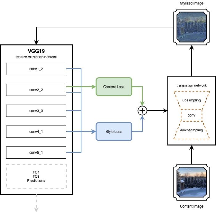
The transformation network is a simple CNN with residual blocks and stride convolutions. Those are used for down and up-sampling within the network.
Conclusion
The translation network is a lightweight CNN that, once trained, can stylize an image in a single feed-forward pass. The much deeper and more complex VGG19 network is no longer needed after training and doesn’t need to be applied to the edge device. This makes style transfer a candidate that can even run on smartphones, especially on those that come with specialized neural hardware like current iPhones and Android devices.
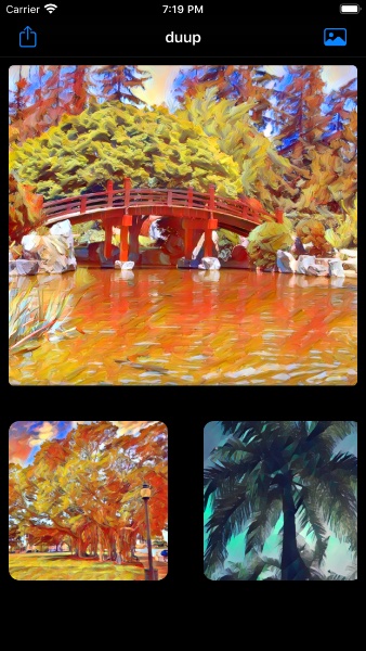
duup
One really nice app that comes with a clear UI design and very nice styles is duup. The app is available for iOS on the app store for free and provides a good feeling for what style transfer can do with your own pictures. I suggest you give it a try and see for yourself.